Compute property
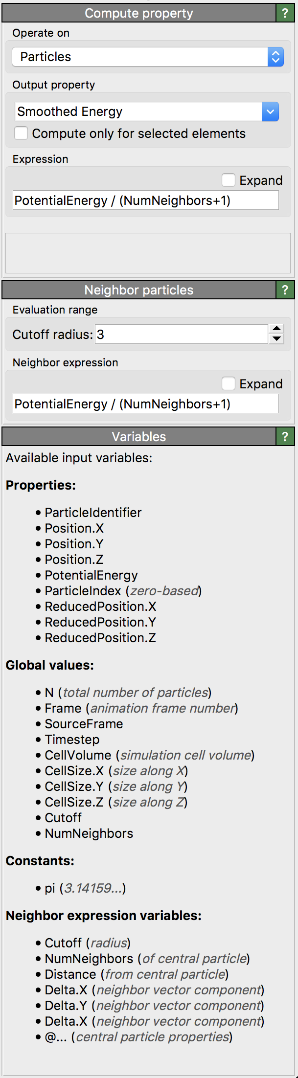
The Compute Property modifier sets property values of particles, bonds, and other elements according to a user-defined mathematical formula. It can also be used to create new user-defined properties.
The math expression for computing the value for each element can reference existing per-particle or per-bond data, as well as global parameters such as the simulation box dimensions or the current animation time. A list of available input variables is provided in the modifier’s user interface. Additionally, the Compute Property modifier supports computations involving neighboring particles within a defined spherical volume around each particle or which are bonded to the central particle.
The output property
As explained in the introduction on particle properties, certain properties, such as Color or Radius,
have special significance within OVITO because they control the visual appearance of individual particles and bonds. Modifying these properties using
the Compute Property modifier directly impacts visualization.
For example, you can:
Modify the
Positionproperty to move particles.Assign new values to the
Colorproperty to recolor particles dynamically.Modify the
Selectionproperty, creating a selection set like the Expression selection modifier, but with greater flexibility.
Additionally, you can create entirely new properties and use them in subsequent operations within the data pipeline or export them to an output file. To do so, simply enter a custom property name in the Output property field. Note that property names in OVITO are case-sensitive. Standard property names predefined by the software are available in the drop-down list.
Vectorial properties
Some particle properties, such as Position and Color, consist of multiple components (XYZ and RGB).
When computing such vector properties, you need to specify a separate scalar expression for each component.
Since OVITO 3.12.1, the modifier also supports the creation of user-defined vector properties. To define a custom vector property, simply enter the names of the vector components into the Components field as a comma-separated list, e.g. “X, Y, Z” and press Enter. The GUI panel will then dynamically display a corresponding number of input fields for you to specify an expression for each component.
Selective assignment
If the specified output property already exists, the modifier overwrites it with the newly computed values. However, by enabling the Compute only for selected option, you can restrict property assignment to a subset of particles or bonds, preserving existing values for currently unselected elements.
Conditional values
You can also use conditional logic within expressions using the ternary operator ? :. This allows for simple if-else conditions.
For example, to make the particles in the upper half of the simulation box semi-transparent while keeping those in the lower half fully opaque,
use the following expression to set the Transparency property of all particles:
(ReducedPosition.Z > 0.5) ? 0.7 : 0.0
For more complex computations that cannot be performed using conditional expressions like this, consider using a Python script modifier, which allows scripting in a real programming language.
Performing computations over neighbors and bonded particles
The Compute Property modifier supports computations that involve the local neighborhood of particles.
The final output value for the \(i\)-th particle is computed as a sum of two terms: a base expression, \(F(i)\), that is evaluated for the central particle \(i\), and a second term, \(G(i,j)\), that is evaluated for each neighboring (or connected) particle \(j\):
\(P(i) = F(i) + \sum_{j \in \mathcal{N}_i}{G(i,j)}\)
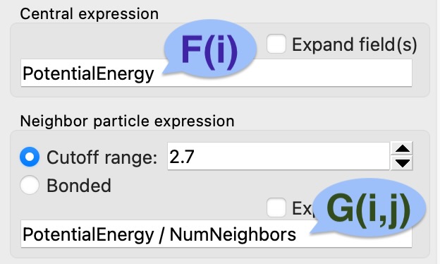
The expressions for \(F(i)\) and \(G(i,j)\) must be entered separately in the user interface of the modifier.
The set of visited neighbors, \(\mathcal{N}_i\), may be defined in two ways:
By specifying a cutoff radius, \(R_c\), around each particle, within which neighboring particles are considered:
\(\mathcal{N}_i = {j: |\mathbf{r}_i - \mathbf{r}_j| < R_c}\),
By using the bonds between particles. The neighbor term will then be evaluated for each particle that has a bond to the current central particle.
The neighbor term \(G(i,j)\) may depend on property values of the current neighbor \(j\), the central particle \(i\), and the vector connecting the two particles.
Example: Smoothing a property over neighboring particles
The neighbor expression allows you to perform advanced computations that involve the local neighborhood of particles. For example, you
can smooth an existing particle property (e.g. InputProperty) by averaging its value over a particle’s local neighborhood:
F(i)   := InputProperty / (NumNeighbors+1)
G(i,j) := InputProperty / (NumNeighbors+1)
NumNeighbors is a dynamic variable yielding the current number of neighboring particles within the selected cutoff radius, ensuring proper normalization.
Example: Lennard-Jones potential calculation
The following expressions compute the potential energy of each particle using a Lennard-Jones function:
F(i)   := 0
G(i,j) := 4 * (Distance^-12 - Distance^-6)
The dynamic variable Distance in the \(G(i,j)\) expression yields the current separation between the central particle and its neighbor.
Example: Counting neighbor particles of a certain type
The \(G(i,j)\) expression may refer to property values of the central particle \(i\) by prepending
the @ prefix to a property name. For instance, the following expressions count the neighbors whose types are
different from the type of the central particle:
F(i)   := 0
G(i,j) := (ParticleType != @ParticleType)
Note that the operator != evaluates to 1 if the type of particle \(j\) is not equal to the type of particle \(i\), and 0 otherwise.
Computations on bonds
The modifier can also operate on bonds instead of particles. Then it will compute a new property for each pair-wise bond in the system.
If Operate on is set to Bonds, expression variables refer to existing per-bond properties.
You can also include properties of the two connected particles by prefixing their property names with @1. or @2..
For example, to select all bonds that connect different particle types and have a length greater than 2.8,
you can set the output bond property to Selection and use the following expression:
@1.ParticleType != @2.ParticleType && BondLength > 2.8
Since bond orientation is arbitrary, @1. and @2. may refer to either connected particle.
Thus, to explicitly select bonds between type-1 and type-2 particles, a more complex expression is necessary
to account for the two possibilities:
(@1.ParticleType == 1 && @2.ParticleType == 2) || (@1.ParticleType == 2 && @2.ParticleType == 1)
Expression syntax
The modifier’s expression syntax resembles that of the C programming language. Variable names and function names are case-sensitive.
Attention
Spaces in property names are simply left out in the corresponding variable names. For example, the particle property Particle Type is accessible as the variable
ParticleType in the expression. Other invalid characters in property names are replaced by underscores in the variable names.
Operators are evaluated in the following order of precedence:
Operator |
Description |
|---|---|
|
Parentheses for explicit precedence |
|
Exponentiation (A raised to the power B) |
|
Multiplication and division |
|
Addition and subtraction |
|
Comparisons between A and B (yielding either 0 or 1) |
|
Logical AND: True if both A and B are non-zero |
|
Logical OR: True if A, B, or both are non-zero |
|
Conditional (ternary) operator: If A differs from 0, yields B, else C |
The expression parser supports the following functions:
Function name |
Description |
|---|---|
|
Absolute value of A. If A is negative, returns -A, otherwise returns A. |
|
Arc-cosine of A. Returns the angle, measured in radians, whose cosine is A. |
|
Same as |
|
Arc-sine of A. Returns the angle, measured in radians, whose sine is A. |
|
Same as |
|
Arc-tangent of A. Returns the angle, measured in radians, whose tangent is A. |
|
Two-argument variant of the arctangent function. Returns the angle, measured in radians. see here. |
|
Same as |
|
Returns the average of all arguments. |
|
Cosine of A. Returns the cosine of the angle A, where A is measured in radians. |
|
Same as |
|
Exponential of A. Returns the value of e raised to the power A where e is the base of the natural logarithm, i.e. the non-repeating value approximately equal to 2.71828182846. |
|
Returns the floating-point remainder of A/B (rounded towards zero). |
|
Rounds A to the closest integer. 0.5 is rounded to 1. |
|
Natural (base e) logarithm of A. |
|
Base 10 logarithm of A. |
|
Base 2 logarithm of A. |
|
Returns the maximum of all values. |
|
Returns the minimum of all values. |
|
Returns: 1 if A is positive; -1 if A is negative; 0 if A is zero. |
|
Sine of A. Returns the sine of the angle A, where A is measured in radians. |
|
Same as |
|
Square root of A. |
|
Returns the sum of all parameter values. |
|
Tangent of A. Returns the tangent of the angle A, where A is measured in radians. |
The parser supports the following constants in expressions:
Constant name |
Description |
|---|---|
|
Pi (3.14159…) |
|
Infinity (∞) |
Type names in expressions
Added in version 3.12.0.
Particle types and bond types are represented by unique numeric identifiers in OVITO, i.e., the ParticleType variable evaluates to an integer value
uniquely identifying the type of the current particle. The same applies to other typed properties
in OVITO such as the Structure Type property.
Each type may have a human-readable name associated with it, e.g., the numeric type 1 may be named “Cu”.
You can use these type names in expressions, e.g., ParticleType == "Cu", where the type name is enclosed in double quotes.
For further information on the use of type names in expressions, see here.
Additional examples
Example: Computing particle speed
To compute the linear velocity (speed) of each particle based on the components \((v_x, v_y, v_z)\) of its velocity vector, you can use the following expression:
sqrt(Velocity.X^2 + Velocity.Y^2 + Velocity.Z^2)
See also
ovito.modifiers.ComputePropertyModifier (Python API)