Bader charge integration pro
Added in version 3.16.0.
This modifier performs Bader charge analysis by integrating a density field defined on a voxel grid. It identifies Bader volumes and assigns the integrated density values from each region to individual atoms.
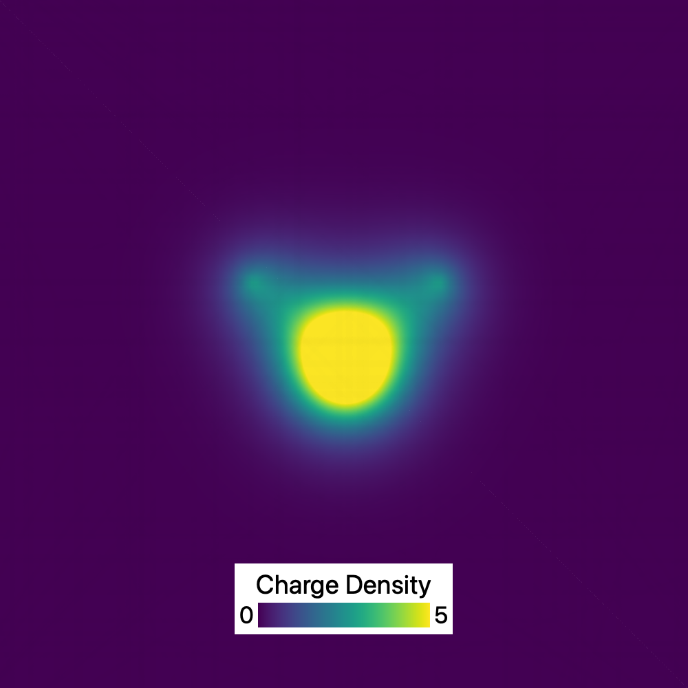
The input charge density field of a H2O molecule, computed using a DFT calculation and imported into OVITO as a voxel grid. This picture shows a 2D slice through the 3D grid.
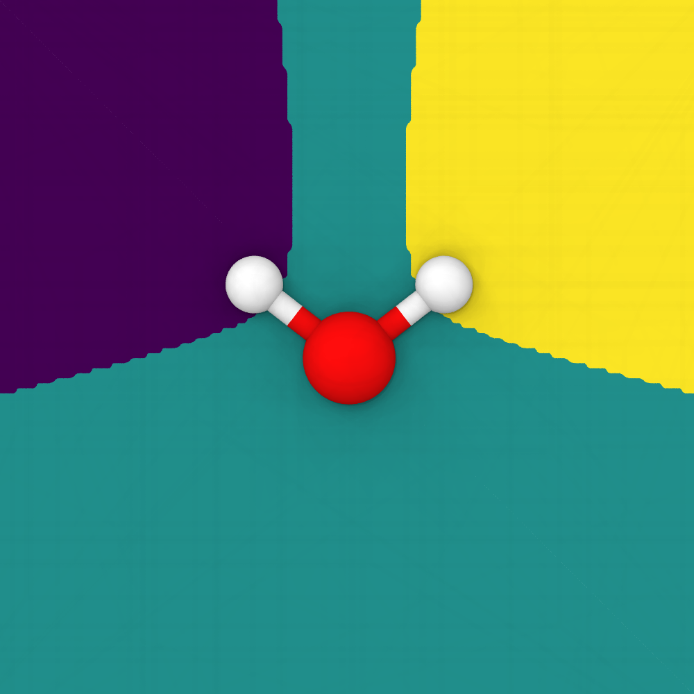
The identified Bader regions, each associated with the atom closest to the local maximum of the density field. The atomic charges are obtained by integrating the charge density over each Bader volume.
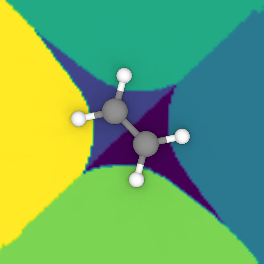
The Bader regions computed by the modifier for a more complex molecule.
The implementation follows the weight method described in:
Please cite this paper when you use this modifier in your work.
Overview
Bader’s theory partitions real space into non-overlapping volumes, each containing a single local maximum of a scalar field (typically the electron charge density). These regions, called Bader volumes or basins of attraction, are bounded by zero-flux surfaces where the gradient of the density has no component normal to the surface:
Here, \(\rho(\vec{r})\) is the density and \(\hat{n}\) is the unit vector perpendicular to the dividing surface at any surface point. Each Bader volume \(\Omega_\rho\) is defined by the set of points whose gradient-ascent trajectory \(\dot{\vec{x}}(t) = \nabla\rho(\vec{x})\) converges to the same unique local maximum.
This modifier identifies Bader volumes in a density field imported into OVITO as a discrete voxel grid. Then it integrates the selected field quantity over each volume to obtain an aggregate value for that region, such as the total charge contained in the Bader volume. Furthermore, if your current dataset contains particles (atoms), the modifier maps each Bader volume to its nearest atom and sums up the integrated quantities per atom, yielding per-atom quantities such as atomic Bader charges and atomic volumes.
Inputs
The modifier requires you to specify the following inputs:
- Voxel grid
A voxel grid with at least one scalar field property, which must represent a density. The grid is typically imported from a DFT calculation (e.g., a CHGCAR file from VASP). The algorithm is limited to regular 3D grids.
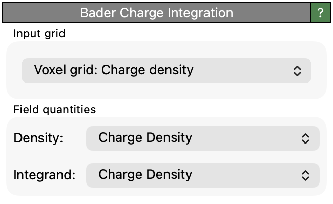
- Density property
Selects the voxel grid property to be used for Bader volume partitioning. The gradient of this field defines the basins of attraction. Typically, this is the electron charge density.
- Integrand property
Selects the scalar voxel grid property to be integrated over each Bader volume. This can be the same as the density property (for computing Bader charges) or a different quantity, e.g., magnetic moments.
Note
The density and integrand properties must be floating-point valued (32-bit or 64-bit). If the integrand property is a multi-component vector field, the modifier integrates each field component separately.
Attention
When using charge density output from VASP, be aware that the standard CHGCAR file only contains the
valence charge density. Since most pseudopotentials remove charge from atomic centers, the Bader
analysis of valence-only densities may not yield physically meaningful atomic charges. For PAW calculations,
add LAECHG=.TRUE. to the INCAR file to have VASP write the core charge density (AECCAR0) and
the valence charge density (AECCAR2) separately. Sum these (using for example the Compute property modifier in OVITO)
to obtain the all-electron charge density per voxel grid cell before performing the Bader analysis. Alternatively you can add in the
known core charge to the integrated valence charges determined by this modifier. In this case, only the per-atom outputs
are physically meaningful and should be used.
- Particles (optional)
If the input dataset contains particles, the modifier maps each identified Bader region to its nearest atom and accumulates the integrated quantities (density, volume, and integrand) as new per-particle properties.
Outputs
The modifier produces the following outputs:
- Bader integration results table
A data table named Bader charge integration listing one row per identified Bader region. Each row contains:
Integrated Density: The integral of the density property over the Bader volume.
Integrated Volume: The volume of the Bader region.
Integrated <Integrand>: The integral of the selected integrand property over the Bader volume (only when the selected integrand property differs from the density property).
Position: The Cartesian coordinates of the density maximum associated with this Bader region.
Mapped Particle Distance: The distance from the density maximum to the nearest atom (only when particles are present).
Mapped Particle Index: The 0-based index of the nearest atom to the maximum (only when particles are present).
- Per-atom properties
When the input dataset contains particles, the modifier assigns the following new particle properties:
Integrated Density: The total integrated density associated with the atom (sum over all Bader regions mapped to that atom).
Integrated Volume: The total Bader volume associated with the atom (sum over all Bader regions mapped to that atom).
Integrated <Integrand>: The total integrated value of the integrand property for the atom (only when the integrand property differs from the density).
- Per-voxel properties
The modifier adds the following new cell properties to the selected voxel grid:
Region: An integer index identifying which Bader region each voxel belongs to (always the region with the maximum weight if the voxel is at the boundary between regions).
Maximum Region Weight: The fractional weight of the dominant region at each voxel.
Mapped Particle Index: The 0-based index of the atom associated with the voxel’s Bader region (only when particles are present).
Algorithm
The modifier uses the weight method of Yu and Trinkle, which assigns fractional volume weights to each grid point rather than performing a binary assignment of grid points to basins.
Weighted integration
For each grid point \(X\), the algorithm computes a weight \(w_A(X)\) between 0 and 1 for each basin \(A\), satisfying \(\sum_A w_A(X) = 1\). The integral of a function \(f(\vec{r})\) over a basin \(A\) is then approximated as:
where \(V_X\) is the volume of the Voronoi cell surrounding grid point \(X\). The weight \(w_A(X)\) represents the fraction of points in the Voronoi cell \(V_X\) whose gradient-ascent trajectory ends in basin \(A\). For interior grid points (where all neighbors with higher density belong to the same basin), the weight is exactly 1 for that basin. Only at boundary grid points (adjacent to multiple basins) do fractional weights arise.
Flux computation
The weights are derived from the probability flux between neighboring grid cells. Starting from a uniform probability density inside the Voronoi cell of grid point \(X\), the flux of probability from \(V_X\) to a neighboring cell \(V_{X'}\) through their shared facet \(\partial V_{X \to X'}\) is:
Here, \(a_{X \to X'}\) is the area of the shared Voronoi facet, \(\ell_{X \to X'}\) is the distance between \(X\) and \(X'\), \(\rho_X\) is the density at grid point \(X\), and \(R(u) = u\,\theta(u)\) is the ramp function (equal to \(u\) when \(u > 0\) and zero otherwise). The ramp function ensures that flux only flows toward neighbors with higher density. The fluxes are normalized such that \(\sum_{X'} J_{X \to X'} = 1\), unless \(X\) is a local density maximum.
Weight propagation
With the fluxes known, the weights for each basin are determined by forward substitution. The grid points are sorted from highest to lowest density and processed sequentially. For each grid point \(X\), the weight for basin \(A\) is computed from the weights of its uphill neighbors:
where the sum runs only over neighbors \(X'\) with \(\rho(X') > \rho(X)\). At a local maximum, \(w_A(X) = 1\) for the new basin \(A\).
See also
ovito.modifiers.BaderChargeIntegrationModifier (Python API)